Coding branch predictors in VHDL

Posted on 2026-08-12

1. The VHDL language
   1. Crash course
   2. Use on Linux
2. Why do we predict branches?
   1. What is a branch?
   2. Pipelining
3. How do we predict branches?
   1. Simplest designs
   2. Saturating counters
   3. Two-level predictor
   4. Hybrid predictors
4. It was all pure speculation...

---

Do you like CPU stuff? I sure do. Personally I find them to be fascinating piece of technology, where every little aspect has been optimized and scaled to its near limit.
There are many techniques that make a CPU ever faster outside of just increasing the clock speed. One of them, which always bogged me, is branch predictors. How does a CPU even predicts the future?

No, it's not using some kind of advanced neural network. This technology predates everything in that matter! Today we'll try to understand how a branch predictor works and simulate it in VHDL.
My information mainly comes from the Wikipedia article on the subject. I find it really good, check it out!

# The VHDL language

# Crash course

VHDL is a Hardware Description Language, that is, it describes how hardware such as CPUs and FPGAs are built and configured respectively.

When programming in VHDL, we define entities which represent black boxes where we have a given set of inputs and a given set of outputs. For example, let's create an adder summing two 4 bits number together:

library IEEE;
use IEEE.STD_LOGIC_1164.ALL;

entity Adder is
  port(
    en: in STD_LOGIC; -- enable --
    a: in STD_LOGIC_VECTOR(3 downto 0);
    b: in STD_LOGIC_VECTOR(3 downto 0);
    s: out STD_LOGIC_VECTOR(3 downto 0)
  );
end entity;

An input/output of type STD_LOGIC simply represents a 0 or 1, low or high.^[1] A vector represents multiple STD_LOGIC values grouped together, for example an 8-bit number can be represented as an STD_LOGIC_VECTOR(7 downto 0).

With the entity defined above, we implemented the following black-box:

       Adder
     +--------+
-----+ en     |
     |        |
==/4=+ a    s +=/4==
     |        |
==/4=+ b      |
     +--------+

Finally, we need to implement the actual working of our black-box. With only what we've written above, we can't do much. There's an "adder" but, it currently does nothing!
There are two main ways to define a behavior in VHDL, called an architecture: structurally and "behavioraly". The first way describes how the entity is done, the second describes what it does.

architecture Structural of Adder is
  -- NOTE: We don't use carries(4)
  signal carries: STD_LOGIC_VECTOR(4 downto 0);
  component fa_1b is
    port(
      a: in STD_LOGIC;
      b: in STD_LOGIC;
      c: in STD_LOGIC;

      sum: out STD_LOGIC;
      carry: out STD_LOGIC
    );
  end component fa_1b;
begin
  carries(0) <= '0';
  gen_port: for i in 0 to 3 generate
    tmp: fa_1b port map(
      a => a(i),
      b => b(i),
      c => carries(i),

      sum => s(i),
      carry => carries(i+1)
      );
  end generate;
end architecture;

Here the "Structural" way is quite convoluted. We first define a component -- think of it like an entity used as an argument -- which is a full adder for 1 bit (hence fa_1b). We then "copy-paste" it 4 times with a for generate loop, which is a way of generating hardware multiple times.
In each anonymous (named tmp) 1-bit full adder, we link their respective inputs to the Adder input, and do the same for their output. As you can see, all of this is very convoluted, fa_1b's code isn't even present here!

You can understand why describing every single connection and wire (signal represents wires) can be daunting and heavy. The big advantage of HDLs is that they allow you to write code in the "Behavioral" way:

use IEEE.NUMERIC_STD.ALL;

architecture Behavioral of Adder is
begin
  s <= STD_LOGIC_VECTOR(signed(a) + signed(b));
end architecture;

As you can see, it's much simpler to understand the code this way. Such simple line is called an implicit process. It is in its nature asynchronous, that is, whenever one of its inputs updates, the output updates as well. In this manner, VHDL resembles a declarative language. The order we define our instructions does not define the control flow.

Sometimes the function can't be easily described in one or two lines, this is especially true with functions which depend on a clock. In those case, they are encapsulated in what is called a process. A process is basically a function which takes as parameters a list of signal it is sensitive to, that is, it will only be called if one of these inputs is updated.

Here is a very minimal synchronous 8-bit counter to give you an example:

entity Counter is
  port(
    clk: in STD_LOGIC;
    count: out STD_LOGIC_VECTOR(7 downto 0)
  );
end entity;

architecture Behavioral of Counter is
  -- the unsigned type is used for arithmetic
  -- STD_LOGIC_VECTOR can't do arithmetic, think of it like an array
  signal count_val: unsigned(7 downto 0);
begin
  update: process(clk)
  begin
    if rising_edge(clk) then
      count_val <= count_val + to_unsigned(1, 8);
    end if;
  end process;

  -- note that this operation is "simple", so it doesn't need a process
  count <= STD_LOGIC_VECTOR(count_val);
end architecture;

Think of a signal as a local variable. It can also be used to represent wires between different inputs and outputs.

Note that the program will use rising edges, that is, a clock signal is detected when going from low to high.

Finally, once our entity and its corresponding architecture has been created, we can test it through a testbench. It is a specialized piece of code which empirically tests many combinations. Then it is up to the developer to verify whether the good output is produced.

# Use on Linux

You might want to try VHDL yourself and potentially the pieces of code I will give below. In those cases I recommend to install the following packages (the line below is VoidLinux specific):

sudo xbps-install -Su ghdl gtkwave make

I did not find any resource to easily automate the job of ghdl, which I find quite clunky. However, I managed to create somewhat of a Makefile that abstracts most of the details:

GHDL ?= ghdl
OUTPUT ?= fst

# Analyze a vhdl file
%.a: %.vhd
	$(GHDL) -a $<

# Run the TestBench
%_tb: %
	$(GHDL) -r $@ --$(OUTPUT)=$@.$(OUTPUT) --stop-time=$(LENGTH)

clean:
	-rm *.vcd *.wave *.fst 2>/dev/null
	-rm work-obj*.cf
.PHONY: clean

Once this is done, you "just" have to define the recipes for an entity and its associated testbench. For example:

SaturatingCounter: sat_counter.a
SaturatingCounter_tb: export LENGTH=80ns # tests run for a given amount
SaturatingCounter_tb: sat_counter_tb.a   # of time, hence "export"

Running make SaturatingCounter_tb will create an associated file (here ending in .fst) which represents the simulation. You then open it with GTKWave to view the emitted signals.

# Why do we predict branches?

# What is a branch?

First of all, let's clarify what a branch is. A branch is anything in the program which alters its flow of instructions. The perfect example is the if statement in C. It can take the first path, or the second, we don't know in advance.

Here is a simple program to compute the factorial^[2] of a number:

typedef unsigned int uint; /* quicker to write */

uint factorial(uint n) {
  if (n < 2)
    return 1;
  else
    return n * factorial(n - 1); /* we use recursion here */
}

We see here that, unless n is small, we always take the second path. We can't know for sure what n is going to be but generally, it's bigger than 1. This represents a branch that we could try to predict!

It can seem kind of far-fetched to try predicting the future for speed's sake. After all, this seems to be quite a complicated task! Why is it even important in the first place? It comes to one of the other very important optimization techniques of the CPU, pipelining.

By the way, you don't have to understand pipelining to understand branch prediction. You can skip the following section if you wish.

# Pipelining

Pipelining? I know that! It's when I'm building my Vulkan shader and it-

This would deserve its own article, and it does on Wikipedia of course x). Here's a link to it just in case you want to know more. Worry not, I'm still going to give you a brief overview.

Let's go for a quick analogy.

Suppose you're wishing to wash some clothes with modern appliances. You've got three steps for every pile of clothes you have: a washing machine, a dryer, and an iron.
You can't dry unwashed clothes and you can't iron wet clothes, so every step is constrained by the one before.

We are going to represent a pile of clothes P through time in the x-axis and action in the y-axis. Here's a normal cycle on a little diagram:

  1 2 3  <-- step number
W P        |
D   P      | the pile is falling through
I     P    v
^-- current action

1. Wash the pile P
2. Dry the pile P
3. Iron the pile P

We could also resume the "W-D-I" process as a single black box "X" which does everything from start to finish.

Now, what happens if we have another pile of clothes Q coming through? Well we can't handle it! We're already too busy processing our pile P through "X". Even if we're ironing our clothes and the washing machine is empty, we can only start Q once we finished with P.
Let's even add a new pile R to our diagram!

  1 2 3 4 5 6 7 8 9
W P     Q     R
D   P     Q     R
I     P     Q     R

This sure seems like a lot of waste! Outside of being visibly overworked, we aren't efficiently using all the nice appliances we have at our disposal.

As you might have guessed, the fix to this issue is what is called pipelining! Our pipeline is the "W-D-I" process where every step is separated and processed independently, in order.
So while P is ironing, we can start drying Q and washing R!

Our updated diagram now looks like this:

  1 2 3 4 5
W P Q R
D   P Q R
I     P Q R

This only required 5 steps instead of 9!

And this is how pipelining works in CPUs. Instead of a washing-drying-ironing cycle, the general steps are referred as fetch-decode-execute. A pipeline can be very deep, much more than 3 steps. Sometimes there are dozen of steps!

So branch prediction lets us speed the process. While we aren't sure the next pile is to be washed, we'll start it anyways based on our guess so we don't have to wait the result of our condition.

Branch prediction tries to keep the pipeline as filled as possible.

# How do we predict branches?

# Simplest designs

The simplest way to predict branches is to not predict them at all! One very concrete application of this statement is for backward branches. A backward branch is just a jump back in the code, for example, a loop!^[3]

unsigned int acc = 1; /* accumulator */
do {
  if (n < 2)
    break;
  acc *= n;
  n -= 1;
} while (true); /* loop back */

So in the example above, if (n < 2) is a forward branch while while (true) is a backward branch. Loops always imply backward branches, and the purpose of a loop is to repeatedly execute a given piece of code.
It makes sense to assume that they'll always loop back, most of the time that's what they're made for. So that's a first way of "predicting" a branch.

For this article, we won't actually implement this predictor. I hope you understand how such simple predictors can still be effective.

# Saturating counters

Saturating counters are exactly what they're named after, a counter which saturates after a given value. For example, if we have a saturating counter from 1 to 3, adding 1 to it while it is at 3 still keeps it at 3.

This can be represented as a finite state machine quite easily, for example a 2-bit saturating counter can take 4 states: strongly not taken, weakly not taken, weakly taken, and strongly taken.

    +------+    +------+    +------+    +------+
+-->|      |-t->|      |-t->|      |-t->|      |-t-+
|   |  SNT |    |  WNT |    |  WT  |    |  ST  |   |
+-n-|      |<-n-|      |<-n-|      |<-n-|      |<--+
    +------+    +------+    +------+    +------+

Here a t represents a "taken" branch while a n represents a "not taken" branch.

With this technique, you basically add friction to changes made in a condition. If a condition almost always match but does not once in a while, the state of the FSM will alternate between WT and ST.

I hope that you can see how such dynamic predictor can be useful, while still being extremely simple. It only requires 2 bits of data and an associated little logic circuit.

Now, let's implement this circuit!

entity SaturatingCounter is
  port (
    clk, rst: in STD_LOGIC;
    taken: in STD_LOGIC;
    pred: out STD_LOGIC
  );
  -- default count correspond to "weakly not taken"
  constant DEF_COUNT: unsigned(1 downto 0) := to_unsigned(1, 2);
end entity;

First, we'll make our black-box or entity. As most things present in CPUs, this logic circuit needs to be synchronous, that is, it depends on a clock which periodically switches between high and low. We will thus have a clk logic input, and a rst logic input for resetting the counter.
Finally, based on the outcome of our last condition named taken, we want to emit a prediction pred. The branch will either be taken or not.
DEF_COUNT is a 2-bit value which is 1, corresponding to the WNT state above.

With all of this in place, we have this black-box corresponding to all our branch predictors:

     Branch
     Predictor
    +---------+
--^-+ clk     |
    |         |
----+ taken   |
    |    pred +----
----+ rst     |
    +---------+

I don't know if this is a common thing to do, but this is how I usually implement my FSMs in VHDL: first make a synchronous process which updates the state, then an asynchronous process which sets the output depending on the state.
Let's define our architecture with a signal used for computation:

architecture Behavioral of SaturatingCounter is
  signal count: unsigned(1 downto 0) := DEF_COUNT;
begin

Then we'll do the easiest thing. If our count is less than 2, the branch is predicted to not be taken. Our FSM is either in the SNT or WNT state.

  ret: process(count) -- we only care about count
  begin
    -- we can access count like an array, it is an STD_LOGIC_VECTOR
    if count(1) = '0' then
      pred <= '0';
    else
      pred <= '1';
    end if;
  end process;

Finally, let's implement the heart of our FSM. While we could have defined four different states for it, we'll just use integers and check them instead.^[4]

  update: process(clk, rst)
  begin
    if rst = '1' then
      count <= DEF_COUNT;
    elsif rising_edge(clk) then
      if taken = '1' and count /= "11" then
        count <= count + 1;
      elsif taken = '0' and count /= "00" then
        count <= count - 1;
      end if;
    end if;
  end process;

So if the branch is taken and we're not in the ST state, we increment our counter. The same logic is applied in the opposite way when decrementing our counter. Finally, when the reset line is high, we go back to our default count.

Changing the value of DEF_COUNT can greatly impact the performance depending on the condition being tested.

How should we build our testbench now? It's technically only a counter so we need to put taken in a high state for long enough, then put it in a low state.

First we define a testbench entity, by convention I end it with _tb. It does not need to have any input or output, as it is purely a simulated concept. We only look at its state through the signals it outputs.

library IEEE;
use IEEE.STD_LOGIC_1164.ALL;

entity SaturatingCounter_tb is end;

Then we have to do the big part of a test bench. First, we declare a component which is the entity we want to test. Remember, using a component is just like an entity we use as an argument.

architecture Behavioral of SaturatingCounter_tb is
  component SaturatingCounter is
    port (
      clk, rst: in STD_LOGIC;
      taken: in STD_LOGIC;
      pred: out STD_LOGIC
    );
  end component;

Then we'll define the signals we want to monitor or change. These signals are basically like the wires we'll act upon, either by measuring them or by putting current in them.

  signal sig_clk: STD_LOGIC := '0'; -- has a default value of '0'
  signal sig_rst, sig_taken, sig_pred: STD_LOGIC;
begin

We instantiate an entity of SaturatingCounter named "uut" for Unit Under Test. To each port it has, we plug one of our defined signals in it. This will allow us to act upon this entity similar to a black-box.

  uut: SaturatingCounter port map(
      clk   => sig_clk,
      rst   => sig_rst,
      taken => sig_taken,
      pred  => sig_pred
  );

Finally, we define how we want to change our inputs. First we'll reset quickly by switching sig_rst to high for 3ns. Our clock is defined with a period of 10ns by switching every 5ns.
Then comes the most important part: sig_taken. We first activate for 40ns, long enough for us to see if the counter saturates. Then, we'll deactivate it for the rest of the simulation. Here it is 80ns long.

  sig_clk <= not sig_clk after 5 ns;
  sig_rst <= '1', '0' after 3 ns;
  sig_taken <= '1', '0' after 40 ns;
end;

It seems that everything is good to go. Let's test it now and see if our basic predictor works well!

make SaturatingCounter_tb
gtkwave SaturatingCounter_tb.fst&

With the chronogram given above, we can see that the count is indeed initialized to 1 -- or the WNT state -- when rst is high. Then the counter gradually increases until saturating to 3 -- or the ST state. We then test for its decrease by putting taken to 0 for a long enough period.
Sure enough, everything appears to work just as expected. Wonderful!^[5]

So that's how a quite simple branch predictor works, let's get to the next level then shall we?

# Two-level predictor

# Working principle

Here is something that I find really clever and impressive, two-level predictors. These are predictors which have an history, keeping track of the n last branch jumps by whether they've been taken or not.
Depending on the history size, this allows the predictor to keep track of complex patterns and predict them perfectly.
What if my branch is taken twice, not taken once, taken once, then not taken three times?^[6] Seems a pretty annoying thing to predict right? Such predictor can handle it!

So, we know it has history, but how so exactly? Suppose our predictor has an history depth of 3bits, it thus has 8 total pattern possibilities kept in a pattern table. The predictor keeps track of the last 3 bits of information by whether branches have been taken or not^[6].

          Pattern
          Table
         +---------+
         | SatCnt0 |
         +---------+
  +----->| SatCnt1 |---> prediction
  |      +---------+
 001     |    .    |
 ---     |    .    |
 branch  |    .    |
 history +---------+
         | SatCnt7 |
         +---------+

Every entry in the pattern table has a saturating counter which for a given bit pattern, predicts whether the branch is taken or not. Using this method, every bit pattern that can fit in our history depth can be tracked and predicted.

# Small example

You might not have perfectly understood how the above mechanism works, that's perfectly fine, it's still a little abstract. Let's go for an example, as a reminder: a branch that is taken is represented by a 1, a branch that is not taken by a 0.

Here we have the following repeating pattern where each period is separated by a |. Whether the branch is taken is written on the first line while the index is written on the second line.

1 0 0 0 1 0 1 1|1 0 0 0 1 0 1 1 ...
0 1 2 3 4 5 6 7 8 9 a b c d e f ...

That's quite a messy pattern. To follow along, we'll think of the branch history as a sliding window (think of it as a basket) which gradually explores the pattern.

First, we don't have enough data to fill our window so we don't change anything. Remember that by default, the saturating counters are in the WNT state.

b 1 0 0 0 1 0 1 1|1 0 0 0 1 0 1 1 ... <- b for branch
i 0 1 2 3 4 5 6 7 8 9 a b c d e f ... <- i for index
1 /                                   <- a number corresponds
2 --/                                    to the current step

After the third step, we have enough data to fill our basket:

b 1 0 0 0 1 0 1 1|1 0 0 0 1 0 1 1 ...
3 \---/ <- the current branch history

We see that after 100 comes a zero, the branch is not taken. So we decrement our saturating counter located in the pattern table at index 100. It comes from the WNT to the SNT state.

Then we continue with the next step:

b 1 0 0 0 1 0 1 1|1 0 0 0 1 0 1 1 ...
4   \---/

After three zeroes in a row comes a one. We increment our saturated counter at index 000 from the WNT to the WT state.

Just a last one before summing it up:

b 1 0 0 0 1 0 1 1|1 0 0 0 1 0 1 1 ...
5     \---/

At index 001 we see a zero, so we do the same move as index 100: decrement the saturating counter moving it from WNT to SNT. This whole method here is presented for a 3-bit history, but you can easily extend it to any depth by widening the "basket".

If we iterate enough times, the counters will converge to these states:

0	1	2	3	4	5	6	7
ST	SNT	ST	ST	SNT	ST	SNT	SNT

We're quite lucky here. All our counters cleanly converged and did not alternate between one or more states. This could have happened if for example the first time the branch was not taken instead of taken.

Increasing the history depth would have solved this issue, but it comes as an exponential cost. This takes 8x2=16 bits for a 3-bit depth, 32 bits for a 4-bit depth etc. Remember that we are inside the CPU itself, the memory and size are much more constrained that what we're used to.

Now that we understand how this more advanced branch predictor works, we can implement it in VHDL!

# Implementation

As it is a branch predictor it will roughly have the same shape as our SaturatingCounter. The definition of the entity thus does not change... at the exception of a powerful little keyword: generic.

library IEEE;
use IEEE.STD_LOGIC_1164.ALL;
use IEEE.NUMERIC_STD.ALL;

entity TwoLevelPredictor is
  generic(
    -- maximum depth of 16
    HIST_DEPTH: natural range 2 to 16 := 2
  );
  port(
    clk, rst: in STD_LOGIC;
    taken: in STD_LOGIC;
    pred: out STD_LOGIC
  );
end entity;

generic allows us to define an entity which can accept a parameter which will change its shape or inner working. Here, this allows us to change the history depth value HIST_DEPTH. The way a two-level predictor works is the same for all history depths.

This time for the implementation, it's a bit more involved. First, we can reuse what we built for the saturating counters! We'll specify that we require a SaturatingCounter as a used component. We also write a constant to have the number of counters we need at hand.

architecture Behavioral of TwoLevelPredictor is
  component SaturatingCounter is
    port (
      clk, rst: in STD_LOGIC;
      taken: in STD_LOGIC;
      pred: out STD_LOGIC
    );
  end component;
  constant CNT_NUM: natural := 2**HIST_DEPTH;

Then we need to keep track of the branch history. This is declared as an unsigned value and not an STD_LOGIC_VECTOR because we will perform logic operations on its value. We also need a small counter to keep track of how many bits were recorded in the history. If you recall in our above example, the first two steps were dismissed due to the incomplete branch history.

  signal hist: unsigned(HIST_DEPTH-1 downto 0) := (others => '0');
  signal len: natural range 0 to HIST_DEPTH := 0;

The (others => '0') idiom is a simple way to set a bunch of units -- such as STD_LOGIC_VECTOR or unsigned -- to zero.^[7]

Finally, we'll add all the wires needed to link the many SaturatingCounter the two-level predictor has. We'll index into them with the sig_idx signal which is just the reintepreted value of hist.^[8]

  signal clks, takens, preds: STD_LOGIC_VECTOR(CNT_NUM-1 downto 0);
  signal sig_idx: natural range 0 to CNT_NUM;

Once all of this is done, we can start implementing the behavior itself. First we generate all the counters and wire them with our signals defined above. This is the simplest part of our architecture, as it only creates our counters.

begin
  gen_cnts: for i in 0 to CNT_NUM-1 generate
    cnt_i: SaturatingCounter port map(
      rst => rst,
      clk => clks(i),     -- this is where we wire each counter
      taken => takens(i), -- input and output to its associated
      pred => preds(i)    -- signal
    );
  end generate;

Then, remember, this is a synchronous entity. This means that we need a process that depends on the clock signal (and the reset one as well). We'll simply name it update as the one shown before.

We check if the reset line is pulled high. If so, we reset all our inner states. ^[9]

  update: process(clk, rst)
  begin
    if rst = '1' then
      hist <= (others => '0');
      takens <= (others => '0');
      clks <= (others => '0');
      len <= 0;

We update our signals by using the value hist and converting it to an integer which is sig_idx. Note that the parenthesis around a value mean that we're accessing it as an "array".

    elsif rising_edge(clk) then
      -- only update when we've acquired enough history
      if len = HIST_DEPTH then
      -- first update the counters
        takens(sig_idx) <= taken;
        clks(sig_idx) <= clk;
      else
        len <= len + 1;
      end if;

      -- then update the history
      hist <= hist(HIST_DEPTH-2 downto 0) & taken;

Using our previously defined SaturatingCounter lets us abstract all the ugly details! It's just a matter of accessing one in particular and giving it a signal. The role of our array above is akin to one of a multiplexer. We also update our history by shifting it to the left and concatenating the taken value. That's what the & operator is for, it does not mean a bitwise AND as in C-based languages.

Once this done, to avoid any issue, we reset the signals sent to our counters to 0. This is done by watching for a falling edge instead of a rising one, that is, when the voltage goes from high to low.

    elsif falling_edge(clk) then
      takens <= (others => '0');
      clks <= (others => '0'); 
    end if;
  end process;

Then, we simply assign our index value and the prediction accordingly. As these are implicit processes, there is no issue in defining them right at the bottom of the architecture.

  sig_idx <= to_integer(hist);
  pred <= preds(sig_idx);
end;

To quicly sum up, what did we just do here?

• We declared some signals to keep track of our branch history and use it as an index
• We declared a bunch of signals which would let us do wiring between our saturated counters
• Then we actually generated those counters
• When rst is high, we simply put everything to 0
• When clk is rising, we update our saturating counters and the branch history accordingly
• On a falling clk, we take care of cleaning every remnant signal
• Our prediction corresponds to the one made by the SaturatingCounter for our current branch history

Few! That sure was a lot. Personally, it took me some time to really get it. I experimented a lot to get exactly how this was working.

Ready? We have to test it then!

# Testing our predictor

Let's reproduce our previous example in the testbench. This probably is the best way to illustrate our predictor's behavior.

As before, we have define an empty entity. Everything that actually defines it is present in our architecture, such as the multiple signals we'll monitor and update. We also import our TwoLevelPredictor as a component.

library IEEE;
use IEEE.STD_LOGIC_1164.ALL;

entity TwoLevelPredictor_tb is end;

architecture Behavioral of TwoLevelPredictor_tb is
  signal sig_clk: STD_LOGIC := '0';
  signal sig_rst, sig_taken, sig_pred: STD_LOGIC;
  signal count: natural;
  component TwoLevelPredictor is
    generic(
      HIST_DEPTH: natural range 1 to 16 := 2
    );
    port(
      clk, rst: in STD_LOGIC;
      taken: in STD_LOGIC;
      pred: out STD_LOGIC
    );
  end component;
begin

Then we instantiate our component which will be our UUT. Here we map the different ports but we map the generics as well. In this case, we only have to set the value of HIST_DEPTH to 3.

  uut: TwoLevelPredictor
  generic map(
    HIST_DEPTH => 3
  )
  port map(
    clk   => sig_clk,
    rst   => sig_rst,
    taken => sig_taken,
    pred  => sig_pred
  );

Finally, as usual, we set our clock to have a period of 10ns and our reset to be high for 3ns. Then we write the process which will be responsible of our weird conditional branch behavior.

  sig_clk <= not sig_clk after 5 ns;
  sig_rst <= '1', '0' after 3 ns;

  update: process(sig_clk)
  begin
    if rising_edge(sig_clk) then
      count <= (count + 1) mod 8;
    end if;

    if count = 0 or count = 4 or count >= 6 then
      sig_taken <= '1';
    else
      sig_taken <= '0';
    end if;
  end process;
end;

Let it roll!

make TwoLevelPredictor_tb
gtkwave TwoLevelPredictor_tb.fst&

We see that our entity is much more complex than before. We have our signals but the multiple counters as well, all having their own signals.^[10]

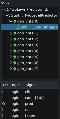
Now that we know this, let's see all of our signals.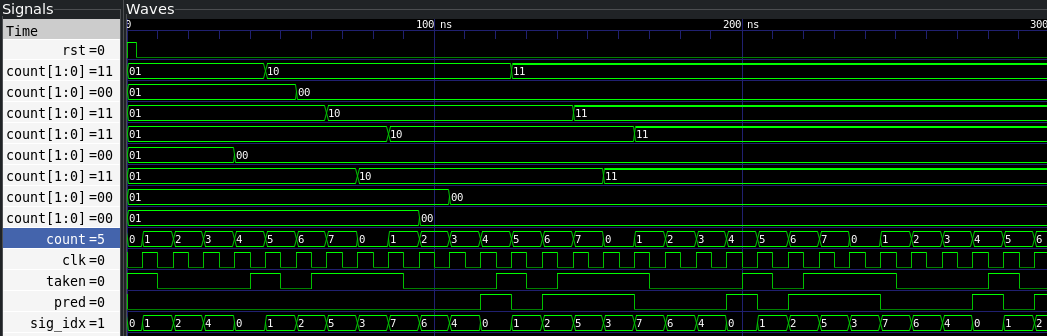

Woa, that's a lot of information to see! I didn't even display anything because we wouldn't be able to understand what's going on anymore. Let's review all of these line by line:

• rst is our reset line, as usual.
• count[1:0] represents the state for a saturating counter. All of these are displayed from top to bottom going from 0 to 7.
• count simply helps us seeing when our period starts and stops
• clk is our clock with a 10ns period.
• taken represents our actual signal to be predicted, it has the exact same shape as the example.
• pred is the prediction made by our branch predictor, it is always half a period ahead of the taken signal
• sig_idx represents the current branch history

We see that first nothing is predicted at all. We don't have enough data for our history to be complete, moreover, the saturating counters are still updating before stabilization.
Then, by looking closer each counter state, we can see them converging after some time. If we assign a name to each of these, we get the following table:

0	1	2	3	4	5	6	7
ST	SNT	ST	ST	SNT	ST	SNT	SNT

It's exactly the same as predicted in the example! We managed to reproduce the behavior of a two-level predictor in VHDL perfectly.

When looking at the pred line, we see that it takes some time, but eventually perfectly predicts the taken line. For this quite messy pattern, the predictor can always guess if the branch will be taken in the next iteration!

# What about misprediction?

I don't know what you think, but I found the previous demonstration simply impressive! We managed to understand the two-level predictor inner working and it works perfectly!

If you remember correctly though, we said that we were quite lucky with this branch pattern. Changing our first "taken" to a "not taken" would effectively mess with the prediction.

b 0 0 0 0 1 0 1 1|0 0 0 0 1 0 1 1 ...
i 0 1 2 3 4 5 6 7 8 9 a b c d e f ...

This is purely because three zeroes can now lead to a zero or a one, so our branch predictor updates its saturating counter constantly!

Updating our program to reproduce this pattern is quite simple:

-    if count = 0 or count = 4 or count >= 6 then
+    if count = 4 or count >= 6 then

With this change, running our program again gives the following chronogram:

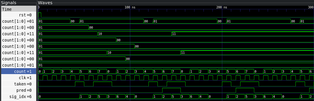
We see especially that the counter 0 always switch between the SNT and WNT states. This results in a slight misprediction for the first jump located at index 4.

For this example though, this is the only issue! Our branch predictor correctly predicts the signal seven times out of eight!

You can find more complex schemes which make it fail more. There are plenty of configurations to test!

# Hybrid predictors

Two-level predictors are really clever in design. With a sufficiant history depth, they are able to predict incredibly complicated schemes! However, this history depth requires exponential growth. Suppose we only wish to predict at most 64 branches in a program, with a 6-bit history. This gives us a total of 64x2x64=8192 bits of storage needed for the predictor only! Memory really isn't cheap inside of the CPU.

There are two main ways to allocate a two-level predictor, either give one to every branch as we calculated before, or share it to all branches. The first scheme is much more reliable but cannot efficiently predict similar schemes for differing branches. These two method are respectively given the attribute local and global.

Remember our very simple loop predictor? We use it for all backward branches while our more complex predictor is used for forward branches. This allows us to more efficiently use our memory, at the cost of a slightly diminished accuracy.

Such schemes are called hybrid predictors, and while I won't implement them here, I found them interesting enough to mention.

# It was all pure speculation...

I hope that you liked this more abstract post. After all, the purpose of this all is only speculation! Our predictors might get things right, or they might fail every single time! Frankly for them to fail every single time it would be a real disaster, designs nowadays are even crazier than the ones shown here.

This technology allowed CPUs to gain significant speed, speculation is now a whole part of the game. It also uncovered a whole class of vulnerabilities such as Spectre and Meltdown.

The entire source code for predictors is available as a gzipped tarball, albeit with slight differences due to it being older than the post itself.

Also, a huge thanks to the Wikipedia article this very post is based on!
I love wandering on Wikipedia and when searching for branch predictors I thought to myself "Ah! How cool it would be to implement it in VHDL!". This explains why, if you read the article, my post shares such a similar structure.

Few, this was a huge post to me. I really hope you liked it and learned something new!

Have a good day!

---